Tutorials
This section contains materials on how to use Eskapade. There are additional side notes on how certain aspects work and where to find parts of the code. For more in depth explanations on the functionality of the code-base, try the API docs.
All command examples below can be run from any directory with write access.
Running your first macro
After successfully installing Eskapade, it is now time to run your very first macro, the classic code example: Hello World!
For ease of use, let’s make shortcuts to the directories containing the Eskapade tutorials:
$ export TUTDIRC=`pip show Eskapade-Core | grep Location | awk '{ print $2"/escore/tutorials" }'`
$ export TUTDIR=`pip show Eskapade | grep Location | awk '{ print $2"/eskapade/tutorials" }'`
$ ls -l $TUTDIRC/ $TUTDIR/
Hello World!
If you just want to run it plain and simple, go to the root of the repository and run the following:
$ eskapade_run $TUTDIRC/esk101_helloworld.py
This will run the macro that prints out Hello World. There is a lot of output, but try to find back these lines (or similar):
2017-11-13T12:37:07.473512+00:00 [eskapade.core_ops.links.hello_world.HelloWorld#INFO] Hello World
2017-11-13T12:37:07.473512+00:00 [eskapade.core_ops.links.hello_world.HelloWorld#INFO] Hello World
Congratulations, you have just successfully run Eskapade!
Internal workings
To see what is actually happening under the hood, go ahead and open up tutorials/esk101_helloworld.py.
The macro is like a recipe and it contains all of your analysis. It has all the ‘high level’ operations that are to be
executed by Eskapade.
When we go into this macro we find the following piece of code:
hello = Chain(name='Hello')
link = core_ops.HelloWorld(name='HelloWorld')
link.logger.log_level = LogLevel.DEBUG
link.repeat = settings['n_repeat']
hello.add(link)
Which is the code that does the actual analysis (in this case, print out the statement). In this case link is an
instance of the class HelloWorld, which itself is a Link. The Link class is the fundamental building block in Eskapade that
contains our analysis steps. The code for HelloWorld can be found at:
$ less python/eskapade/core_ops/links/hello_world.py
Looking into this class in particular, in the code we find in the execute() function:
self.logger.info('Hello {hello}', hello=self.hello)
where self.hello is a parameter set in the __init__ of the class. This setting can be overwritten as can be seen
below. For example, we can make another link, link2 and change the default self.hello into something else.
link2 = core_ops.HelloWorld(name='Hello2')
link2.hello = 'Lionel Richie'
ch.add(link2)
Rerunning results in us greeting the famous singer/songwriter.
There are many ways to run your macro and control the flow of your analysis. You can read more on this in the Short introduction to the Framework subsection below.
Tutorial 1: transforming data
Now that we know the basics of Eskapade we can go on to more advanced macros, containing an actual analysis.
Before we get started, we have to fetch some data, on your command line, type:
$ wget https://s3-eu-west-1.amazonaws.com/kpmg-eskapade-share/data/LAozone.data
To run the macro type on your CLI:
$ eskapade_run $TUTDIR/tutorial_1.py
If you want to add command line arguments, for example to change the output logging level, read the page on command line arguments.
When looking at the output in the terminal we read something like the following:
2017-11-13T13:37:07.473512+00:00 [eskapade.core.execution#INFO] *              Welcome to Eskapade!                *
...
2017-11-13T13:37:08.085577+00:00 [eskapade.core.process_manager.ProcessManager#INFO] Number of registered chains: 2
...
2017-11-13T13:37:11.316414+00:00 [eskapade.core.execution#INFO] *              Leaving Eskapade. Bye!              *
There is a lot more output than these lines (tens or hundred of lines depending on the log level). Eskapade has run the code from each link, and at the top of the output in your terminal you can see a summary.
When you look at the output in the terminal you can see that the macro contains two chains and a few Link are contained in these chains. Note that chain 2 is empty at this moment. In the code of the macro we see that in the first chain that data is loaded first and then a transformation is applied to this data.
Before we are going to change the code in the macro, there will be a short introduction to the framework.
Short introduction to the Framework
At this point we will not go into the underlying structure of the code that is underneath the macro, but later in this
tutorial we will. For now we will take a look in the macro. So open $TUTDIR/tutorial_1.py in your
favorite editor. We notice the structure: first imports, then defining all the settings, and finally the actual
analysis: Chains and Links.
A chain is instantiated as follows:
data = Chain('Data')
and registered automatically with the ProcessManager. The ProcessManager is the main event processing loop and is responsible for processing the Chains and Links.
Next a Pandas data frame converter Link is initialized and its properties are set, and finally added to the data chain:
reader = analysis.ReadToDf(name='Read_LA_ozone', path='LAozone.data', reader=pd.read_csv, key='data')
data.add(reader)
This means the Link is added to the chain and when Eskapade runs, it will execute the code in the Link.
Now that we know how the framework runs the code on a higher level, we will continue with the macro.
In the macro notice that under the second chain some code has been commented out. Uncomment the code and run the macro again with:
$ eskapade_run $TUTDIR/tutorial_1.py
And notice that it takes a bit longer to run, and the output is longer, since it now executes the Link in chain 2. This Link takes the data from chain 1 and makes plots of the data in the data set and saves it to your disk. Go to this path and open one of the pdfs found there:
$ results/Tutorial_1/data/v0/report/
The pdfs give an overview of all numerical variables in the data in histogram form. The binning, plotting and saving of this data is all done by the chain we just uncommented. If you want to take a look at how the Link works, it can be found in:
$ python/eskapade/visualization/links/df_summary.py
But for now, we will skip the underlying functionality of the links.
Let’s do an exercise. Going back to the first link, we notice that the transformations that are executed are defined in conv_funcs passed to the link.
We want to include in the plot the wind speed in km/h. There is already a
part of the code available in the conv_funcs and the functions comp_date and mi_to_km. Use these functions
as examples to write a function that converts the wind speed.
Add this to the transformation by adding your own code. Once this works you can also try to add the temperature in degrees Celsius.
Making a Link
Now we are going to add a new link that we create! To make a new link type the following:
$ eskapade_generate_link --dir python/eskapade/analysis/links YourLink
The command will make a link object named YourLink in the path specified in the first argument.
The link we wish to add will do some textual transformation, so name it accordingly.
And be sure to follow the instructions given by the command!
The command creates the skeleton file:
$ python/eskapade/analysis/links/yourlink.py
This skeleton file can be modified with your custom editor and then be imported and called inside a macro with
analysis.YourLink(). Notice that the name of the class is CamelCase and that the name of the file is lowercase
to conform to coding guidelines.
Now open up the link in your editor.
In the execute function of the Link, we see that a DataStore is called. This is the central in-memory object in
which all data is saved. DataStore inherits from a dict, so by calling the right key we can get objects. Call:
df = ds['data']
to get the DataFrame that includes the latest transformations.
Now we are going to make a completely different transformation in the Link and apply it to the object in the DataStore. We want to add a column to the data that states how humid it is. When column ‘humidity’ is less than 50 it is ‘dry’, otherwise it is ‘humid’. You will have to use some pandas functionality or perhaps something else if you prefer. Save the new column back into the DataFrame and then put the DataFrame in the DataStore under the key ‘data_new’.
We are going to let our plot functionality loose on this DataFrame once more, to see what happens to our generated textual data. It can not be plotted. In the future this functionality will be available for most data types.
Now run the entire macro with the new code and compile the output .tex file. This can be done on the command line with
$ cd results/Tutorial_1/data/v0/report/
$ pdflatex report.tex
If you have pdflatex installed on your machine.
Note
If you don’t have pdflatex installed on your machine you can install it by executing the following command: .. code-block:: bash
$ yum install texlive-latex-recommended
Now take a look at the output pdf. The final output should look something like this:
Your plot should be quite similar (though it might be different in its make up.)
In summary, the work method of Eskapade is to run chains of custom code chunks (links). Each chain should have a specific purpose, for example pre-processing incoming data, booking and/or training predictive algorithms, validating these predictive algorithms, evaluating the algorithms.
By using this work method, links can be easily reused in future projects. Some links are provided by default. For example, links used to load data from a json file, book predictive algorithms, predict the training and test data set and produce evaluation metrics. If you want to use your own predictive model just go ahead and add your own links!
Tutorial 2: macro from basic links
In this tutorial we are going to build a macro using existing Links. We start by using templates to make a new macro. The command
$ eskapade_generate_macro --dir python/eskapade/tutorials tutorial_2
makes a new macro from a template macro. When we open the macro we find a lot of options that we can use. For now we will actually not use them, but if you want to learn more about them, read the Examples section below.
First we will add new chains to the macro. These are the higher level building blocks that can be controlled when starting a run of the macro. At the bottom of the macro we find a commented out Link, the classic Hello World link. You can uncomment it and run the macro if you like, but for now we are going to use the code to make a few chains.
So use the code and add 3 chains with different names:
ch = Chain('CHAINNAME')
When naming chains, remember that the output of Eskapade will print per chain-link combination the logs that are defined in the Links. So name the chains appropriately, so when you run the macro the logging actually makes sense.
This tutorial will be quite straight-forward, it has 3 short steps, which is why we made 3 chains.
- In the first chain: Read a data file of your choosing into Eskapade using the pandas links in the analysis subpackage.
- In the second chain: Copy the DataFrame you created in the DataStore using the core_ops subpackage.
- In the third chain: Delete the entire DataStore using a Link in the core_ops subpackage.
To find the right Links you have to go through the Eskapade documentation (or code!), and to find within its subpackages
the proper Links you have to understand the package structure.
Every package is specific for a certain task, such as analysis, core tasks (like the ProcessManager), or data
quality. Every subpackage contains links in its links/ subdirectory.
See for example the subpackages core_ops, analysis or visualization.
In All available examples we give some tips to find the right Links your analysis, and how to configure them properly.
Tutorial 3: Jupyter notebook
This section contains materials on how to use Eskapade in Jupyter Notebooks. There are additional side notes on how certain aspects work and where to find parts of the code. For more in depth explanations, try the API-docs.
Next we will demonstrate how Eskapade can be run and debugged interactively from within a Jupyter notebook.
An Eskapade notebook
To run Eskapade use the eskapade_generate_notebook command to create a template notebook. For example:
$ eskapade_generate_notebook --dir ./ notebook_name
The minimal code you need to run a notebook is the following:
from eskapade import process_manager, resources, ConfigObject, DataStore
from eskapade.core import execution, persistence
from eskapade.logger import LogLevel

# --- basic config
settings = process_manager.service(ConfigObject)
settings['macro'] = resources.tutorial('tutorial_1.py')
settings['version'] = 0
settings['logLevel'] = LogLevel.DEBUG

# --- optional running parameters
# settings['beginWithChain'] = 'startChain'
# settings['endWithChain'] = 'endChain'
# settings['resultsDir'] = 'resultsdir'
settings['storeResultsEachChain'] = True

# --- other global flags (just some examples)
# settings['set_mongo'] = False
# settings['set_training'] = False

# --- run eskapade!
execution.eskapade_run(settings)

# --- To rerun eskapade, clear the memory state first!
# execution.reset_eskapade()
Make sure to fill out all the necessary parameters for it to run. The macro has to be set obviously, but not all
settings in this example are needed to be set to a value. The function execution.eskapade_run(settings) runs
Eskapade with the settings you specified.
To inspect the state of the Eskapade objects (datastore and configurations) after the various chains see the command line examples below. .. note:
Inspecting intermediate states requires Eskapade to be run with the option storeResultsEachChain
(command line: ``-w``) on.
# --- example inspecting the data store after the preprocessing chain
ds = DataStore.import_from_file('./results/Tutorial_1/proc_service_data/v0/_Summary/eskapade.core.process_services.DataStore.pkl')
ds.keys()
ds.Print()
ds['data'].head()

# --- example showing Eskapade settings
settings = ConfigObject.import_from_file('./results/Tutorial_1/proc_service_data/v0/_Summary/eskapade.core.process_services.ConfigObject.pkl')
settings.Print()
The import_from_file function imports a pickle file that was written out by Eskapade, containing the DataStore.
This can be used to start from an intermediate state of your Eskapade. For example, you do some operations on your
DataStore and then save it. At a later time you load this saved DataStore and continue from there.
Running in a notebook
In this tutorial we will make a notebook and run the macro from tutorial 1. This macro shows the basics of Eskapade. Once we have Eskapade running in a terminal, we can run it also in Jupyter. Make sure you have properly installed Jupyter.
We start by making a notebook:
$ eskapade_generate_notebook tutorial_3_notebook
This will create a notebook in the current directory with the name tutorial_3_notebook running
macro tutorial_1.py. You can set a destination directory by specifying the command argument --dir.
Now open Jupyter and take a look at the notebook.
$ jupyter notebook
Try to run the notebook. You might get an error if the notebook can not find the data for the data reader. Unless
you luckily are in the right folder. By default, tutorial_1.py looks for the data file LAozone.data in
the working directory. Use:
!pwd
In Jupyter to find which path you are working on, and put the data to the path. Or change the load path in the macro to the proper one. But in the end it depends on your setup.
Intermezzo: you can run bash commands in Jupyter by prepending the command with a !
Now run the cells in the notebook and check if the macro runs properly. The output be something like:
2017-02-14 14:04:55,506 DEBUG [link/execute_link]: Now executing link 'LA ozone data'
2017-02-14 14:04:55,506 DEBUG [readtodf/execute]: reading datasets from files ["../data/LAozone.data"]
2017-02-14 14:04:55,507 DEBUG [readtodf/pandasReader]: using Pandas reader "<function _make_parser_function.<locals>.parser_f at 0x7faaac7f4d08>"
2017-02-14 14:04:55,509 DEBUG [link/execute_link]: Done executing link 'LA ozone data'
2017-02-14 14:04:55,510 DEBUG [link/execute_link]: Now executing link 'Transform'
2017-02-14 14:04:55,511 DEBUG [applyfunctodataframe/execute]: Applying function <function <lambda> at 0x7faa8ba2e158>
2017-02-14 14:04:55,512 DEBUG [applyfunctodataframe/execute]: Applying function <function <lambda> at 0x7faa8ba95f28>
2017-02-14 14:04:55,515 DEBUG [link/execute_link]: Done executing link 'Transform'
2017-02-14 14:04:55,516 DEBUG [chain/execute]: Done executing chain 'Data'
2017-02-14 14:04:55,516 DEBUG [chain/finalize]: Now finalizing chain 'Data'
2017-02-14 14:04:55,517 DEBUG [link/finalize_link]: Now finalizing link 'LA ozone data'
2017-02-14 14:04:55,518 DEBUG [link/finalize_link]: Done finalizing link 'LA ozone data'
2017-02-14 14:04:55,518 DEBUG [link/finalize_link]: Now finalizing link 'Transform'
2017-02-14 14:04:55,519 DEBUG [link/finalize_link]: Done finalizing link 'Transform'
2017-02-14 14:04:55,519 DEBUG [chain/finalize]: Done finalizing chain 'Data'
with a lot more text surrounding this output. Now try to run the macro again. The run should fail, and you get the following error:
KeyError: Processor "<Chain name=Data parent=<... ProcessManager ...> id=...>" already exists!'
This is because the ProcessManager is a singleton. This means there is only one of this in memory allowed, and since the Jupyter python kernel was still running the object still existed and running the macro gave an error. The macro tried to add a chain, but it already exists in the ProcessManager. Therefore the final line in the notebook template has to be ran every time you want to rerun Eskapade. So run this line:
execution.reset_eskapade()
And try to rerun the notebook without restarting the kernel.
execution.eskapade_run(settings)
If one wants to call the objects used in the run, execute contains them. For example calling
ds = process_manager.service(DataStore)
is the DataStore, and similarly the other ‘master’ objects can be called. Resetting will clear the process manager singleton from memory, and now the macro can be rerun without any errors.
Note: restarting the Jupyter kernel also works, but might take more time because you have to re-execute all of the necessary code.
Reading data from a pickle
Continuing with the notebook we are going to load a pickle file that is automatically written away when the engine runs. First we must locate the folder where it is saved. By default this is in:
./results/$MACRO/proc_service_data/v$VERSION/latest/eskapade.core.process_services.DataStore.pkl'
Where $MACRO is the macro name you specified in the settings, $VERSION is the version you specified and
latest refers to the last chain you wrote to disk. By default, the version is 0 and the name is v0 and the chain is
the last chain of your macro.
You can write a specific chain with the command line arguments, otherwise use the default, the last chain of the macro.
Now we are going to load the pickle from tutorial_1.
So make a new cell in Jupyter and add:
from eskapade import DataStore
to import the DataStore module. Now to import the actual pickle and convert it back to the DataStore do:
ds = DataStore.import_from_file('./results/Tutorial_1/proc_service_data/v0/latest/eskapade.core.process_services.DataStore.pkl')
to open the saved DataStore into variable ds. Now we can call the keys of the DataStore with
ds.Print()
We see there are two keys: data and transformed_data. Call one of them and see what is in there. You will find
of course the pandas DataFrames that we used in the tutorial. Now you can use them in the notebook environment
and directly interact with the objects without running the entirety of Eskapade.
Similarly you can open old ConfigObject objects if they are available. By importing and calling:
from eskapade import ConfigObject
settings = ConfigObject.import_from_file('./results/Tutorial_1/proc_service_data/v0/latest/eskapade.core.process_services.ConfigObject.pkl')
one can import the saved singleton at the path. The singleton can be any of the above mentioned stores/objects.
Finally, by default there are soft-links in the results directory at results/$MACRO/proc_service_data/$VERSION/latest/
that point to the pickles of the associated objects from the last chain in the macro.
Tutorial 4: creating a new analysis project
Now that we have covered how to make a link, macro, and notebook we can create a new analysis project. To generate a new project type the following:
$ eskapade_bootstrap --project_root_dir ./yourproject -m yourmacro -l YourLink --n yournotebook yourpackage
The script will create a Python package called yourpackage in the path specified in the --project_root_dir argument.
The arguments -m, -l, and -n are optional, if not specified the default values are used.
The generated project has the following structure:
|-yourproject
   |-yourpackage
      |-links
         |-__init__.py
         |-yourlink.py
      |-__init__.py
      |-yourmacro.py
      |-yournotebook.ipynb
   |-setup.py
The project contains a link module called yourlink.py under links directory,
a macro yourmacro.py, and a Jupyter notebook yournotebook.ipynb with required dependencies.
To add more of each to the project you can use the commands generate_link, generate_macro, and generate_notebook
like it was done before.
The script also generates setup.py file and the package can be installed as any other pip package.
Let’s try to debug the project interactively within a Jupyter notebook. First, go to your project directory and install the package in an editable mode:
$ cd yourproject
$ pip install -e .
As you can see in the output, installation checks if eskapade and its requirements are installed.
If the installation was successful, run Jupyter and open yournotebook.ipynb in yourpackage directory:
$ jupyter notebook
As you see in the code the notebook runs yourmacro.py:
settings['macro'] = '<...>/yourproject/yourpackage/yourmacro.py'
Now run the cells in the notebook and check if the macro runs properly.
Tutorial 5: Data Mimic
This section contains materials on how to use Eskapade in to re-simulate data. We will explain how to use the links present in the submodule and what choice were made.
Running the macro
To run the tutorial macro enter the command in a shell:
$ eskapade_run $TUTDIR/esk701_mimic_data.py
The tutorial macro illustrates how to resample a dataset using kernel density estimation (KDE). The macro can handle contiunous data, and both ordered and unordered catagorical data. The macro is build up in the following way:
- A dataset is simulated containing mixed data types, representing general input data.
- Some cleaning steps are performed on the dataset
- KDE is applied to the dataset
- Using the estimated bandwidths of the KDE, the data is resampled
- An evaluation is done on the resulting resimulated dataset
We’ll go through each of the links and explain the workings, choices made and available options so to help facitilitate the use after a client engagement.
To run the macro for a client engamgent you need to change out the first link, which simulates fake data, to the ReadToDf link in order to read in the data:
settings['input_path'] = 'diamonds.csv'
settings['reader'] = 'csv'
settings['separator'] = ','
settings['maps'] = maps

np.random.seed(42)

ch = Chain('do_all')

reader = analysis.ReadToDf(name='reader',
                           path=settings['input_path'],
                           sep=settings['separator'],
                           key='df',
                           reader=settings['reader'])
ch.add(reader)
For ordered variables that are strings, it is important that you provide the settings['maps']) variable. It contains a dictonary mapping the string values of the variable to a numeric value that matches the order from low to high. For example, a variable ordered containing ‘low’, ‘medium’ and ‘high’ values should be mapped to 0, 1 and 3. If the mapping is not included the macros will assing numeric values but in order of first appearance, thus not guaranteeing the implied order of the strings. (aka: the macro doesnt know ‘low’ is the lowest, or ‘V1’ is the lowest value in your catagory.)
Warning
When providing the map for ordered catagorical variables, you also need to add them for the unordered catagorical variables which are strings. The macro will either create maps for all string variables, or will use the provided maps input.
Addionally, you need to provide the macro with the data type contained in each column, ordered-, and unordered catagorical, or continuous. Finally also provide the columns which contain strings, so the macro will transfer them to numerical values. In case of ordered catagorical values this will happen using the maps you mentioned above. If it is not provided, the macro will automatically create a map and add it to the datastore. The automatically created map does not take any implicit order of catagories into account.
settings['unordered_categorical_columns'] = ['a','b']
settings['ordered_categorical_columns'] = ['d','c']
settings['continuous_columns'] = ['e','f','g']
settings['string_columns'] = ['a','c']
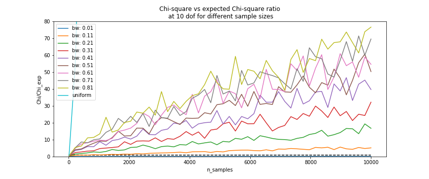
The rest of the macro can be run as is as far as functionality goes. There are a few parameters that can be tweaked to optimize the results:
ds['bw']inResampleris a list of bandwidths estimated by the kde corresponding to the columns of the data as stored inds.binsinResampleEvaluationcontrols the bins used to bin the data for chi square evaluation. For more details on the impact of choosing these bins please refer to Chi-square
Mixed Variables Simulation
The first link exists to create some fake data to run the tutorial macro on. Naturally, if you want to run the data_mimic to resimulate a specific dataset, this link is not necessary.
The link takes some parameters as input that will determine how the data is generated, such as the number of observations, the probabilities associated with each category per dimension, and the mean stds for the coninuous data.
KDE Preperation
- In order to do Kernel Density Estimation we need to prepare the data. This means:
- Converting strings to dummy integer variables and saving the mapping
- Remove any
NaNvalues present - Find peaks in distributions
- Transforms continuous variables to copula space (transform to a normal distribution)
- Performs a PCA transformation (optional)
- Hash column names and variables if required
Each of these transformations are saved to the datastore including their properties needed to transform the data back.
Kernel Density Estimation
This link performs the actual KDE. The link takes the normalized data in case of the continuous variables, and the data without NaN values for catagorical variables. It then applies the KDEMultivariate implementation from statsmodels, using the ‘normal-rule-of-thumb’ for quick calculation.
Note
There is a faster method available if only unordered variables are present. This method is selected automatically.
The result is a bandwidth bw for each variable, which are saved in a list in the datastore.
Resampler
- Currently the resampler loops over each datapoint and variable j and resamples by:
- Resamples a new point from a normal distribution centered at the original datapoint, with
std=bw[j], for continuous varibales. - Resamples randomly from all catagories != current catagory if
bw[j] > np.random.rand()for unordered catagorical variables. - Resamples using a Wang-Ryzin kernel defined at the datapoint using bandwith
bw[j]for ordered catagorical variables.
- Resamples a new point from a normal distribution centered at the original datapoint, with
ResampleEvaluation
Evaluates the distribution similarities based on Chi-square, Kolmogorov-Smirnov and the Cosine distance. The formulas and applications of these metrics to the datset are explained below.
Chi-square
When applying the two sample chi-square test we are testing whether two datasets come from a common distribution.
- \(H_0\): The two sets come from a common distribution
- \(H_1\): \(H_0\) is false, the sets come from different distributions
The Chi-square test we use is calculated using the formula:
where R is the resampled dataset and E the expected values, or in our context, the original dataset.
In case the datasets are not of equal sample size, we can still use the Chi-square test using the scaling constants. If the sets of of equal sample size, the constants will go to 1, and we are left with the ‘traditional’ chi-square formula:
Kolmogorov-Smirnov
The Kolmogorov–Smirnov test may also be used to test whether two underlying one-dimensional probability distributions differ. In this case, we apply the KS test to each variable and save the results.
Note
The KS test assumes the distribution is continuous. Although the test is run for all variables, we should keep this in mind when looking at the results for the catagorical variables.
If the K-S statistic is small or the p-value is high, then we cannot reject the null-hypothesis that the distributions of the two samples are the same. Aka: They are sufficiently similar to say they are from the same distrubution.
Cosine-distance
We also tried to define a distance from the original dataset to the resampled one. We employ the cosine distance applied to each point and its resampled point, represented as a vector. The distance will be 0 when on top of each other, and the max distance is.
- We define a vector as the combination of all variables for one datapoint (or row in your dataset).
- All continuous values are represented as is
- All ordered catagorical values are mapped to numerical values going from 0 to # of catagories available, where 0 corresponds to the lowest ranking catagory.
- All unordered catagorical are ignored for now since we have not yet defined a sufficient distance measure for these.
Then, the cosine distance is calculated for each point and it’s corresponding resample.
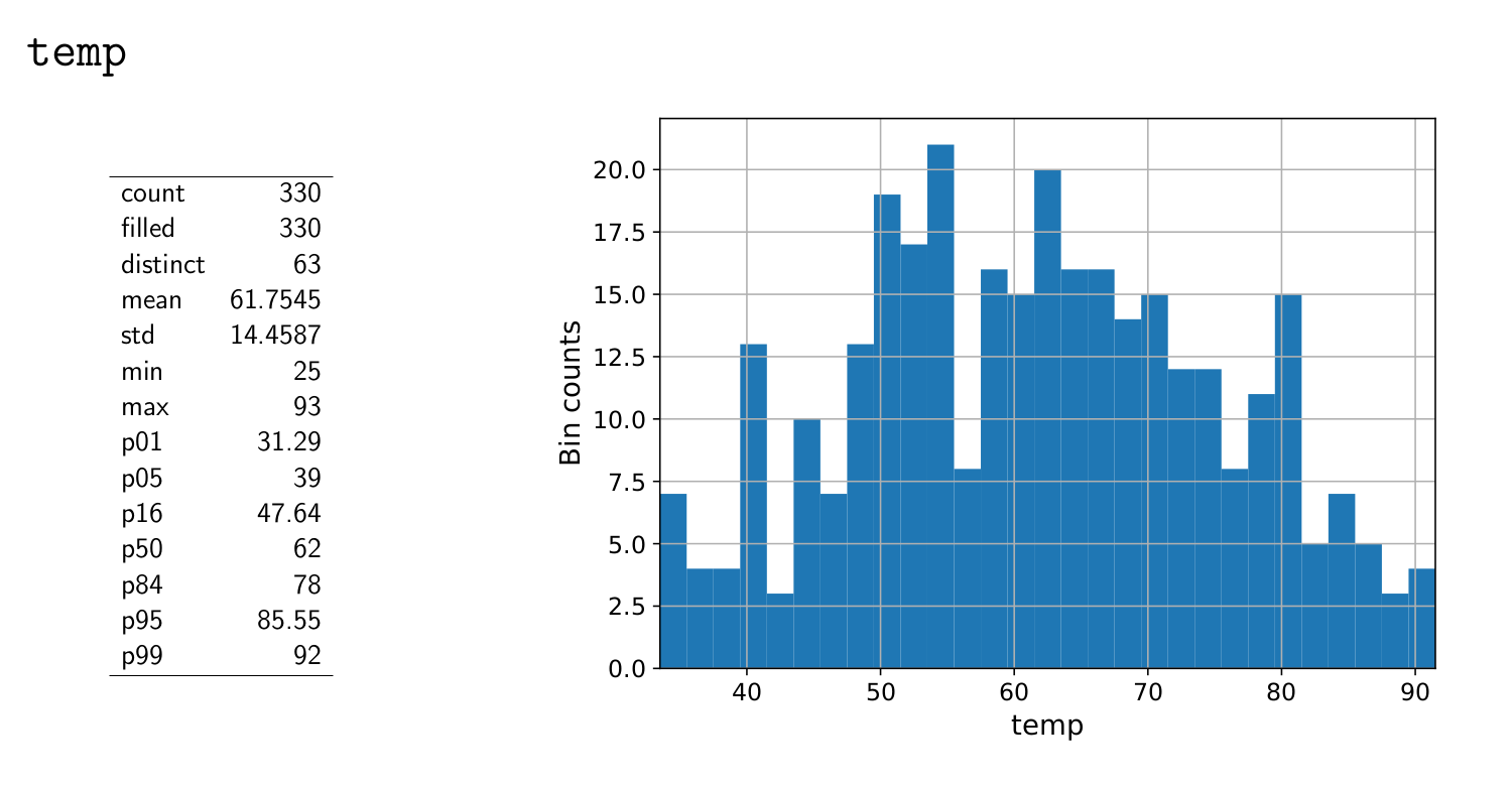
Mimic Report
- The mimic report link will create a standard eskapade style pdf report. The report includes per variable:
- A stacked histogram plot showing before and after the resampling
- A stacked histogram plot of the data per variable in the copula space and a normal distribution
- A correlation matrix of numeric values before and after resimulation
Each variable page also contains the chi-square values comparing before and afer the resampling (also see Chi-square). For each variable, there is a table containing several values. The values correspond the chisquare calculation done on a 1D histogram of the variable itself, and done on 2D histograms of two variables as listed in the table.
Example: On the page of variable d
| Chi2 | p-value | dof | |
|---|---|---|---|
| d | 1.22018 | 0.269325 | 3 |
| e | 1034.82 | 0 | 3 |
| f | 317.124 | 0 | 3 |
| g | 1118.11 | 0 | 3 |
| a | 7.92157 | 0.0476607 | 3 |
| b | 1.4137 | 0.84181 | 3 |
| c | 1.43721 | 0.696837 | 3 |
The value 1.22 corresponds to the calculation variable d before and after the resampling. The value of 1034.82 corresponds to the calculations done on a 2D histogram of variables d and e, before and after the resampling.
Finally, two other metrics, the Kolmogorov-Smirnov and the cosine distance, are also calculated and shown in the report. You can find these on the last page.
All available examples
To see the available Eskapade examples, do:
$ export TUTDIRC=`pip show Eskapade-Core | grep Location | awk '{ print $2"/escore/tutorials" }'`
$ export TUTDIR=`pip show Eskapade | grep Location | awk '{ print $2"/eskapade/tutorials" }'`
$ ls -l $TUTDIRC/ $TUTDIR/
Many Eskapade example macros exist in the tutorials directory. The numbering of the example macros follows the package structure:
esk100+: basic macros describing the chains, links, and datastore functionality of Eskapade.esk200+: macros describing links to do basic processing of pandas dataframes.esk300+: visualization macros for making histograms, plots and reports of datasets.esk500+: macros for doing data quality assessment and cleaning.esk700+: macros for doing data simulation.
The Eskapade macros are briefly described below. They explain the basic architecture of Eskapade, i.e. how the chains, links, datastore, and process manager interact.
Hopefully you now have enough knowledge to run and explore Eskapade by yourself. You are encouraged to run all examples to see what Eskapade can do for you!
Example esk101: Hello World!
Macro 101 runs the Hello World Link. It runs the Link twice using a repeat kwarg, showing how to use kwargs in Links.
$ eskapade_run $TUTDIRC/esk101_helloworld.py
Example esk102: Multiple chains
Macro 102 uses multiple chains to print different kinds of output from one Link. This link is initialized multiple times with different kwargs and names. There are if-statements in the macro to control the usage of the chains.
$ eskapade_run $TUTDIRC/esk102_multiple_chains.py
Example esk103: Print the DataStore
Macro 103 has some objects in the DataStore. The contents of the DataStore are printed in the standard output.
$ eskapade_run $TUTDIRC/esk103_printdatastore.py
Example esk104: Basic DataStore operations
Macro 104 adds some objects from a dictionary to the DataStore and then moves or deletes some of the items. Next it adds more items and prints some of the objects.
$ eskapade_run $TUTDIRC/esk104_basic_datastore_operations.py
Example esk105: DataStore Pickling
Macro 105 has 3 versions: A, B and C. These are built on top of the basic macro esk105. Each of these 3 macro’s does something slightly different:
- A does not store any output pickles,
- B stores all output pickles,
- C starts at the 3rd chain of the macro.
Using these examples one can see how the way macro’s are run can be controlled and what it saves to disk.
$ eskapade_run $TUTDIRC/esk105_A_dont_store_results.py
$ eskapade_run $TUTDIRC/esk105_B_store_each_chain.py
$ eskapade_run $TUTDIRC/esk105_C_begin_at_chain3.py
Example esk106: Command line arguments
Macro 106 shows us how command line arguments can be used to control the chains in a macro. By adding the arguments from the message inside of the macro we can see that the chains are not run.
$ eskapade_run $TUTDIRC/esk106_cmdline_options.py
Example esk107: Chain loop
Example 107 adds a chain to the macro and using a repeater Link it repeats the chain 10 times in a row.
$ eskapade_run $TUTDIRC/esk107_chain_looper.py
Example esk108: Event loop
Example 108 processes a textual data set, to loop through every word and do a Map and Reduce operation on the data set. Finally a line printer prints out the result.
$ source $TUTDIRC/esk108_eventlooper.sh
Example esk109: Debugging tips
This macro illustrates basic debugging features of Eskapade. The macro shows how to start a python session while running through the chains, and also how to break out of a chain.
$ eskapade_run $TUTDIRC/esk109_debugging_tips.py
Example esk110: Code profiling
This macro demonstrates how to run Eskapade with code profiling turned on.
$ eskapade_run $TUTDIRC/esk110_code_profiling.py
Example esk111: Loading a datastore from file
Macro illustrates how to load an external datastore from file.
$ eskapade_run $TUTDIRC/esk111_load_datastore_from_file.py
Example esk201: Read data
Macro 201 illustrates how to open files as pandas datasets. It reads a file into the DataStore. The first chain reads one csv into the DataStore, the second chain reads multiple files (actually the same file multiple times) into the DataStore. (Looping over data is shown in example esk209.)
$ eskapade_run $TUTDIR/esk201_readdata.py
Example esk202: Write data
Macro 202 illustrate writing pandas dataframes to file. It reads a DataFrame into the data store and then writes the DataFrame to csv format on the disk.
$ eskapade_run $TUTDIR/esk202_writedata.py
Example esk203: apply func to pandas df
Illustrates the link that calls basic apply() to columns of a pandas dataframes. See for more information pandas documentation:
http://pandas.pydata.org/pandas-docs/stable/generated/pandas.DataFrame.apply.html
$ eskapade_run $TUTDIR/esk203_apply_func_to_pandas_df.py
Example esk204: apply query to pandas df
Illustrates the link that applies basic queries to pandas dataframe. See for more information pandas documentation:
http://pandas.pydata.org/pandas-docs/stable/generated/pandas.DataFrame.query.html
$ eskapade_run $TUTDIR/esk204_apply_query_to_pandas_df.py
Example esk205: concatenate pandas dfs
Illustrates the link that calls basic concat() of pandas dataframes. See for more information pandas documentation:
http://pandas.pydata.org/pandas-docs/stable/merging.html
$ eskapade_run $TUTDIR/esk205_concatenate_pandas_dfs.py
Example esk206: merge pandas dfs
Illustrate link that calls basic merge() of pandas dataframes. For more information see pandas documentation:
http://pandas.pydata.org/pandas-docs/stable/merging.html
$ eskapade_run $TUTDIR/esk206_merge_pandas_dfs.py
Example esk207: record vectorizer
This macro performs the vectorization of an input column of an input dataframe. E.g. a columnn x with values 1, 2 is tranformed into columns x_1 and x_2, with values True or False assigned per record.
$ eskapade_run $TUTDIR/esk207_record_vectorizer.py
Example esk208: record factorizer
This macro performs the factorization of an input column of an input dataframe. E.g. a columnn x with values ‘apple’, ‘tree’, ‘pear’, ‘apple’, ‘pear’ is tranformed into columns x with values 0, 1, 2, 0, 2.
$ eskapade_run $TUTDIR/esk208_record_factorizer.py
Example esk209: read big data itr
Macro to that illustrates how to loop over multiple (possibly large!) datasets in chunks.
$ eskapade_run $TUTDIR/esk209_read_big_data_itr.py
Example esk210: dataframe restoration
Macro to illustrate writing pandas dataframes to file and reading them back in whilst retaining the datatypes and index using numpy and feather file formats.
$ eskapade_run $TUTDIR/esk210_dataframe_restoration.py
Example esk301: dfsummary plotter
Macro shows how to plot the content of a dataframe in a nice summary pdf file.
(Example similar to $TUTDIR/tutorial_1.py.)
$ eskapade_run $TUTDIR/esk301_dfsummary_plotter.py
Example esk302: histogram_filler_plotter
Macro that illustrates how to loop over multiple (possibly large!) datasets in chunks, in each loop fill a (common) histogram, and plot the final histogram.
$ eskapade_run $TUTDIR/esk302_histogram_filler_plotter.py
Example esk303: histogrammar filler plotter
Macro that illustrates how to loop over multiple (possibly large!) datasets in chunks, in each loop fill a histogrammar histograms, and plot the final histograms.
$ eskapade_run $TUTDIR/esk302_histogram_filler_plotter.py
Example esk304: df boxplot
Macro shows how to boxplot the content of a dataframe in a nice summary pdf file.
$ eskapade_run $TUTDIR/esk304_df_boxplot.py
Example esk305: correlation summary
Macro to demonstrate generating nice correlation heatmaps using various types of correlation coefficients.
$ eskapade_run $TUTDIR/esk305_correlation_summary.py
Example esk306: concatenate reports
This macro illustrates how to concatenate the reports of several visualization links into one big report.
$ eskapade_run $TUTDIR/esk306_concatenate_reports.py
Example esk501: fix pandas dataframe
Macro illustrates how to call FixPandasDataFrame link that gives columns consistent names and datatypes. Default settings perform the following clean-up steps on an input dataframe:
- Fix all column names. Eg. remove punctuation and strange characters, and convert spaces to underscores.
- Check for various possible nans in the dataset, then make all nans consistent by turning them into numpy.nan (= float)
- Per column, assess dynamically the most consistent datatype (ignoring all nans in that column). Eg. bool, int, float, datetime64, string.
- Per column, make the data types of all rows consistent, by using the identified (or imposed) data type (by default ignoring all nans)
$ eskapade_run $TUTDIR/esk501_fix_pandas_dataframe.py
Example esk701: Mimic dataset
Macro that illustrates how to resample a dataset using kernel density estimation (KDE). The macro can handle contiunous data, and both ordered and unordered catagorical data. The macro is build up in the following way:
- A dataset is simulated containing mixed data types, representing general input data.
- Some cleaning steps are performed on the dataset
- KDE is applied to the dataset
- Using the estimated bandwidths of the KDE, the data is resampled
- An evaluation is done on the resulting resimulated dataset
$ eskapade_run $TUTDIR/esk701_mimic_data.py
Example esk702: Mimic data only unordered
This macro illustrates how to resample an existing data set, containing only unordered catagorical data, using kernel density estimation (KDE) and a direct resampling technique.
$ eskapade_run $TUTDIR/esk702_mimic_data_only_unordered.py
Tips on coding
This section contains a general description on how to use Eskapade in combination with other tools, in particular for the purpose of developing code.
Eskapade in PyCharm
PyCharm is a very handy IDE for debugging Python source code. It can be used to run Eskapade stand-alone (i.e. like from the command line) and with an API.
- Stand-alone
- Install PyCharm on your machine.
- Open project and point to the Eskapade source code
- Configuration, in ‘Preferences’, check the following desired values:
- Under ‘Project: eskapade’ / ‘Project Interpreter’:
- The correct Python version (Python 3)
- Under ‘Build, Execution & Deployment’ / ‘Console’ / ‘Python Console’:
- The correct Python version (Python 3)
- Install Eskapade in editable mode
- Run/Debug Configuration:
- Under ‘Python’ add new configuration
- Script: path to the console script
eskapade_run(located in the same directory as the interpreter specified above in ‘Project Interpreter’) - Script parameters: path to a macro to be debugged, e.g.
$ESKAPADE/python/eskapade/tutorials/tutorial_1.py, andeskapade_runcommand line arguments, e.g.--begin-with=Summary - Python interpreter: check if it is the correct Python version (Python 3)
You should now be able to press the ‘play button’ to run Eskapade with the specified parameters.
Writing a new Link using Jupyter and notebooks
Running the framework works best from the command line (in our experience), but running experiments and trying new ideas is better left to an interactive environment like Jupyter. How can we reconcile the difference in these work flows? How can we use them together to get the most out of it?
Well, when using the data and config import functionality of Eskapade together with Jupyter we can interactively work on our objects and when we are satisfied with the results integration into links is straight-forward. The steps to undertake this are in general the following:
- Import the DataStore and/or ConfigObject. Once you have imported the ConfigObject, run it to generate the output you want to use.
- Grab the data you want from the DataStore using
ds = DataStore.import_from_fileanddata = ds[key].- Now you can apply the operation you want to do on the data, experiment on it and work towards the end result you want to have.
- Create a new link in the appropriate link folder using the eskapade_generate_link command.
- Copy the operations (code) you want to do to the link.
- Add assertions and checks to make sure the Link is safe to run.
- Add the Link to your macro and run it!
These steps are very general and we will now go into steps 5, 6 and 7. Steps 1, 2, 3 and 4 have already been covered by various parts of the documentation.
So assuming you wrote some new functionality that you want to add to a Link called YourLink and you have created a new Link from the template we are going to describe how you can get your code into the Link and test it.
Developing Links in notebooks
This subsection starts with a short summary of the workflow for developing Links:
- Make your code in a notebook
- Make a new Link
- Port the code into the Link
- Import the Link into your notebook
- Test if the Link has the desired effect.
- Finish the Link code
- Write a unit test (optional but advised if you want to contribute)
We continue with a longer description of the steps above.
When adding the new code to a new link the following conventions are used:
In the __init__ you specify the key word arguments of the Link and their default values, if you want to get an
object from the DataStore or you want to write an object back into it, use the name read_key and store_key.
Other keywords are free to use as you see fit.
In the initialize function in the Link you define and initialize functions that you want to call when executing the
code on your objects. If you want to import something, you can do this at the root of the Link, as per PEP8.
In the execute function you put the actual code in this format:
settings = process_manager.service(ConfigObject)
ds = process_manager.service(DataStore)

## --- your code follows here
Now you can call the objects that contain all the settings and data of the macro in your Link, and in the code below you can add your analysis code that calls from the objects and writes back in case that this is necessary. Another possibility is writing a file to the disk, for example writing out a plot you made.
If you quickly want to test the Link without running the entire Eskapade framework, you can import it into your notebook sessions:
import eskapade.analysis.links.yourlink
from yourlink import YourLink
l = YourLink()
l.execute()
should run your link. You can also call the other functions. However, execute() is supposed to contain the bulk of your
operations, so running that should give you your result. Now you can change the code in your link if it is not how you
want it to run. The notebook kernel however keeps everything in memory, so you either have to restart the kernel, or
use
import importlib
importlib.reload(eskapade.analysis.links.yourlink)
from yourlink import YourLink
l = YourLink()
l.execute()
to reload the link you changed. This is equivalent to the Python2 function reload(eskapade).
Combined with the importing of the other objects it becomes clear that you can run every piece of the framework from a notebook. However working like this is only recommended for development purposes, running an entire analysis should be done from the command line.
Finally after finishing all the steps you use the function finalize() to clean up all objects you do not want to
save.
After testing whether the Link gives the desired result you have to add the proper assertions and other types of checks into your Link code to make sure that it does not have use-cases that are improperly defined. It is advised that you also write a unit test for the Link, but unless you want it merged into the master, it will not be enforced.
Now you can run Eskapade with your macro from your command line, using the new functionality that you first created in a notebook and then ported into a stand-alone Link.